Solve Sudokus with Convolutional Neural Networks

In this blog post, we explore how to solve Sudokus using convolutional neural networks (CNNs). We will extend the algorithmic approach from the previous post [1] with a neural-network-based component.
We first introduce the model architecture, then discuss the training data, and finally present an algorithm that uses the probabilistic neural model to solve the deterministic, step-by-step Sudoku logic. We analyze the algorithm’s performance and conclude with ideas for future extensions. The code is written in Python using PyTorch and is available on my GitHub.
Training Data
The basic idea is to build a neural network that takes the full grid as input and predicts all empty values simultaneously. Useful information for prediction includes the value of each cell and its allowed values, determined by the constraints of the other cells.
Each cell is encoded as follows:
- Value (one-hot): The cell’s value is one-hot encoded with 10 bits (including an extra bit for empty cells).
Example:
0010000000→ value 2. - Allowed values (one-hot): A 9-bit vector where a bit is 1 if the corresponding value is allowed, 0 otherwise.
Example:
001001001→ allowed values 3, 6, 9.
In total, each cell has 19 channels: 10 for the value and 9 for the allowed values.
The target is the solution value, indexed from 0 to 8 (for 9 classes, used in the cross-entropy loss [2]). We only predict non-filled cells, so we include a mask consisting of bits indicating whether each cell is empty 1 or filled 0.
We use the base dataset [3] containing 3 million Sudoku puzzles along with their solutions and difficulty ratings. In
neural_solve/create_train_data_script.py
we filter out all Sudokus with a rating of 0 and then solve all trivial solutions so that each remaining puzzle is at a stage where the backtracking algorithm from the previous post must start guessing. If a Sudoku can be solved trivially, it is filtered out. We end up with 1,715,919 Sudokus.
From these Sudokus the script creates a CSV file containing the following columns:
- Input: vector of length 81 × 19 = 1,539 (81 cells x 19 channels, values 0 or 1).
- Target: vector of length 81 (values 0–8).
- Mask: vector of length 81 (values 0 or 1).
We implement a PyTorch dataset [4] that reads from the generated CSV in
neural_solve/dataset.py
The dataset produces three tensors: the input tensor x_n_19_81 (dimension N x 19 x 81) containing the Sudoku cells
in
row format (from top left to bottom right), the target
tensor target_n_81 (dimension N x 81), and the mask tensor mask_n_81 (dimension N x 81), where N is the batch
size.
Model
Our input is of dimension N x 19 x 81, and because we predict all values of the Sudoku grid at once, the output must have shape N x (81×9) = N x 729: for each of the 81 cells, we output the probabilities for values 1–9. The simplest approach would be a dense network with 19×81 = 1,539 input neurons and 729 output neurons, with some hidden layers in between. However, such a model would be quite large in terms of the number of weights, making it prone to overfitting and slower in performance.
There is an inherent symmetry in Sudoku: within rows, columns, and boxes, the same rule applies, nine values, each appearing exactly once. The 9 rows, 9 columns, and 9 boxes form 27 so-called Sudoku entities. The idea is as follows: define a subnetwork for each individual entity and share the weights across all subnetworks, since the rules within each entity are identical. Sharing the weights drastically reduces the number of trainable parameters.
There is an elegant way to implement this, borrowed from computer
vision [5]: convolutional neural networks (CNNs).
Let’s start with the row entities. Since the input is already in row format (the 81 cells are ordered so that each
consecutive group of nine represents one row, and the rows follow each other sequentially), we can use
a 1D convolutional neural network with a kernel size of 9, stride 9, and no padding. In
PyTorch [6], this can be
implemented using Conv1d. The convolutional neural network processes all row entities at once and produces an
output of dimension N x FM x 9, where FM is the number of feature maps. This is equivalent to treating each row
entity individually and transforming its 19 x 9 input neurons into FM output
neurons [7]. After the convolutional
layer, a ReLU activation function [8] is
applied. After swapping the last two dimensions, the tensor of shape N x 9 x FM is passed through a linear layer
that maps it to N x 9 x OUT, followed by another ReLU activation function. The whole subnetwork is visualized in the
blog’s title figure.
The model is implemented in
neural_solve/model.py - RowColBox
We can use the same model for the column and box entities. The only difference is that the input must be rearranged so that all cells belonging to the same entity are grouped together consecutively (column / box format), for example, all cells of column / box 0, then all cells of column / box 1, and so on.
Now let’s discuss the full network. In
neural_solve/model.py - SudokuNet
we apply the RowColBox model to rows, columns, and boxes after rearranging the inputs into their corresponding formats. We then concatenate the outputs from all entities, resulting in a tensor of dimension N x (27×OUT). Next, a linear layer produces a tensor of dimension N x DENSE_OUT, followed by another ReLU activation function. DENSE_OUT is another hyperparameter. Finally, a linear layer maps to 9 × 81 = 729 classes, representing the nine possible values for each of the 81 cells.
Training
We use
neural_solve/train_utils.py
to specify the values of all the hyperparameters. The training is implemented in
neural_solve/train_script.py
We split the dataset into training, validation, and test sets. We use 10,000 samples for testing, 40,000 for validation, and the remaining 1,665,919 samples for training. We use the Adam optimizer [9] with a learning rate of 0.0001 and a weight decay of 0.001.
Each empty cell in the Sudoku grid can take a value from 1 to 9, corresponding to class indices 0 to 8. During training, we only want to compute the loss for the empty cells, since the filled cells already contain known values. To achieve this, we use the previously calculated mask to restrict loss computation to positions where the mask equals 1, implemented in
neural_solve/train_utils.py - masked_ce_loss
The model is trained using cross-entropy loss, but instead of using the default mean reduction, we normalize the loss by the number of masked cells. This ensures that the loss is averaged only over relevant predictions.
We evaluated different hyperparameter configurations for the model. A relatively small model with strong performance was achieved using the following values:
FM = 456OUT = 27DENSE_OUT = 729
Note that 456 is a multiple of the 19 input channels, 27 corresponds to the number of Sudoku entities, and 729 represents the number of output neurons.
Training runs efficiently on Apple’s Metal Performance Shaders [10] with a batch size of 1024, using an Apple M2 Max with 96 GB of RAM.
In the plot below, the training and validation losses are shown over the epochs. Both decrease sharply within the first 20 epochs. There is slight overfitting, but since the validation loss continues to decrease, this is acceptable. The large amount of training data and the slim network architecture help prevent severe overfitting.
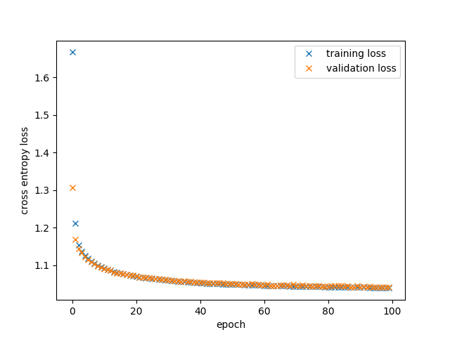
After 100 epochs, the training loss reached 1.039 and the validation loss 1.041. The initial loss was approximately
ln(9) ≈ 2.197, corresponding to the uniform probability over the 9 possible values for an empty cell.
Neural Sudoku Solver Algorithm
So far, we have predicted all empty cells of the Sudoku at once. However, setting a value for one cell imposes constraints on other cells in the same row, column, and block. Since Sudoku is inherently a step-by-step process, predicting all empty cells simultaneously is therefore not an effective approach.
We use the backtracking algorithm developed in [1] to solve the Sudoku. Each time the algorithm needs to make a guess, the neural network is used to predict all empty cells. However, not all of the 81 x 9 outputs from the neural network are valid, since some cells are already filled and some values are disallowed by the constraints imposed by other cells. We use the raw logits and first set all values that are disallowed by the Sudoku constraints to a large negative number. Note that the information about which values are disallowed is already encoded in the 9 allowed-values-channels of the 19-channel training data input. Afterwards, we apply a softmax [11] and obtain probabilities. Then we set all probabilities of non-empty cells to zero. Finally, we select the cell–value combination with the highest probability, that is, the one where the neural network is most confident. This is realized in
neural_solve/get_most_certain_coord_and_index_value.py - get_most_certain_coord_and_index_value
At the corresponding coordinate, we set this value. This defines our neural guess strategy, implemented in
neural_solve/solve.py - neural_guess_strategy
With this algorithm, we can now re-evaluate our training process. When guessing only from the pool of empty cells and allowed values, and selecting the combination in which the neural network is most confident, what success rate do we achieve? In
neural_solve/train_utils.py - validate
this success rate is computed on the validation set. The success rate on the validation set over the training epochs is shown in the figure below.
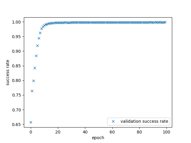
After 12 epochs, it already exceeds 99 %. We reach a maximum success rate of ≈ 99.87 % on the validation set after 89 epochs. With
neural_solve/evaluate_on_test_set_script.py
we evaluate our final model (after epoch 89) on the test set, achieving a success rate of 99.91 %. This shows that the guess strategy is almost always correct, and backtracking is rarely required in the original Sudoku solving algorithm from [1].
In addition to its high accuracy, the model is compact, containing a total of 1,155,111 trainable parameters and occupying 4.6 MB of storage. It can be found under
data/final_sudoku_net_model.pth
Benchmark
In
benchmark/solve_many_sudokus_script.py
we use the 327 non-trivial Sudokus derived from the dataset [12], as in the previous blog post [1], to validate and benchmark the solver with our neural guess strategies.
It takes on average 2.74 ms to solve a Sudoku with our new algorithm. Since a single neural network inference already takes around 0.30 ms, the algorithm cannot outperform classical backtracking strategies. Moreover, while the algorithm’s guesses are almost always correct, it still needs to make many of them. This is because the neural network is often most confident about cells that do not significantly reduce the search space.
Further Ideas
There are several ways to further explore the neural Sudoku solver:
- Since the neural network is highly confident in its predictions, it could make several sequential guesses at once.
- We could focus on guesses that reduce the search space the most. The neural network could be specifically trained on such cases.
- The neural network can process a batch of Sudokus in parallel. The algorithm could therefore be extended to solve multiple Sudokus simultaneously.
- Sudoku symmetries can be exploited. Numbers (1–9) can be relabeled, rows or columns can be permuted within their bands and stacks, and the grid can be rotated or reflected. These symmetries can be used for data augmentation to generate additional training samples.
- In the previous blog post [1], we demonstrated how to generate valid Sudoku grids. In theory, this allows us to create an infinite amount of training data.
Conclusion
We analyzed how to use a Convolutional Neural Network (CNN) to predict empty cells in a Sudoku grid. Our model is relatively small yet achieves high accuracy when focusing on the most confident guesses. Using this model, we developed a neural guess strategy that integrates into the framework introduced in the previous blog post [1]. This demonstrates how a step-by-step process can be approached with a probabilistic machine learning method. However, because inference is computationally expensive, solving Sudokus with the classical backtracking algorithm remains faster from a performance perspective.