Create and Solve Sudokus
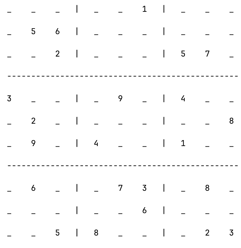
Sudoku is a widely loved logical puzzle, and here we’ll focus on the classic 9x9 variant. The basic rules are explained in [1]. In [2], different techniques are described which people use to solve these puzzles, some of them with interesting names like X-Wing and Swordfish.
Sudokus can also be solved algorithmically. For me, this is a bit nostalgic, since one of my first programming challenges was building a Sudoku solver in Microsoft Excel with VBA (yes, a very long time ago).
In this blog post, we will explore how to solve Sudoku puzzles with algorithms. Once we can solve them, we’ll look at how to generate a random, valid, fully filled Sudoku grid. From there, we’ll see how to create Sudokus with a specified number of clues.
The code is written in Python and can be found on my GitHub. All performance measurements were done on an Apple M2 Max with 96 GB of RAM.
Solve a Sudoku
We model solving immutably: every time a value is set at some coordinate, we create a new state. A state stores the current grid, the last set coordinate, the coordinate’s tries (explained later), and a reference to the previous state. The resulting state graph is effectively a linked list, which we call solution path. Each state in this path is referred to as
solve/solve.py - SolutionPathNode
Each cell has a set of allowed values, meaning the possible numbers it can take. These allowed values are determined by the constraints of the other cells in the same row, column, and block. If a cell has only one allowed value, we refer to it as a trivial solution.
We can use the following recursive approach, implemented in
solve/solve.py - recursively_find_solution
First we solve all trivial solutions until none remain. Then we guess a value at a specific coordinate and restart by solving trivial solutions again.
If we guess a wrong value, the Sudoku will eventually become invalid. In that case, a cell will have no allowed values, meaning we have reached a dead end and must “go back”. This process is called backtracking (see [3]): We return to the last guess we made and try a different value from the set of allowed values. Therefore, each state must keep track of all previously tried values. We could, in principle, guess a value at a completely different coordinate when backtracking, but exploring the limited set of allowed values at a specific coordinate reduces the search space much more effectively than branching over many possible coordinates. If all allowed values of a cell have been tried and each one leads to a dead end, we must backtrack further to the previous guess, and continue this process as needed.
There are several methods to determine at which coordinate to guess a value when no trivial solutions remain. We call this the guess strategy. One option is to choose a coordinate at random, implemented in
solve/solve.py - random_guess_strategy
The algorithm can also guess the coordinate in a fixed order. For example, by scanning the cells from top left to bottom right (row format) and selecting the next empty cell. This is implemented in
solve/solve.py - ordered_guess_strategy
Another approach is to choose the coordinate with the smallest number of allowed values, since guessing there reduces the search space the most. This is the preferred strategy for solving a Sudoku and is implemented in
solve/solve.py - smallest_allowed_guess_strategy
The final algorithm for solving a Sudoku is implemented in
solve/solve.py - solve_grid
We use the dataset [4] to validate and benchmark the solver with different guess strategies. Out of the one million Sudoku puzzles in the dataset, only 327 are non-trivial, meaning they require at least one step of guessing. Since there is randomness in the solver (for example, when selecting a value or when picking a coordinate in the random guess strategy), we solve each puzzle multiple times.
Across strategies, solving takes about 0.30 ms on average per Sudoku. However, the standard deviation for 100 runs is too high to allow a meaningful comparison. While the strategy that chooses the coordinate with the fewest allowed values requires less backtracking, it also has to loop over all coordinates to find the optimal one. In contrast, the random and ordered strategies select coordinates much faster, but backtrack more often. These effects appear to balance each other out. It is therefore expected that for more complex Sudokus requiring more guesses, the smallest allowed strategy will perform best.
Create a Filled Sudoku
Creating a filled Sudoku grid is essentially the same problem as solving an empty Sudoku. We choose the random guess strategy to generate grids with high entropy. During creation, however, the algorithm can get stuck exploring unfruitful search branches. We define depth to increase by one each time the algorithm tries a new value at a coordinate. The minimum depth for creating a filled Sudoku is 81, meaning only one-shot solutions without backtracking are possible. To avoid wasting time in unpromising branches, we set a maximum depth. Once this limit is reached, the creation process restarts from the beginning. The final algorithm to create a valid, filled, and random Sudoku grid is implemented in
solve/solve.py - create_filled
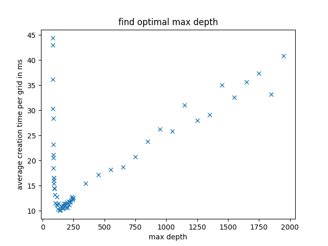
In the graph below, we see the average execution time for generating a filled grid at different maximum depths. The graph was created by generating 100 Sudokus at each maximum depth and calculating the average time. Allowing the algorithm to backtrack reduces creation time significantly, while larger maximum depths cause it to get stuck in unfruitful branches, leading to longer runtimes. For future experiments, we choose a maximum depth of 150, which brings the creation time for a filled Sudoku grid down to about 10 ms.
Create a Sudoku
First, we create a filled Sudoku grid as described above. The idea is to then remove values from the grid one by one until we reach the desired number of clues. A valid Sudoku must always have exactly one unique solution. Each time we remove a value, there is a chance that multiple solutions become possible, although at least one solution always exists since we started from a valid filled grid. Therefore, after every removal we must check that the solution remains unique.
The algorithm to check whether a Sudoku has a unique solution is again recursive:
create/create.py - check_if_has_unique_solution
First, we solve all trivial solutions until none remain. Then we use the smallest-allowed strategy to determine which coordinate to handle, since the search space for potential alternative solutions is smallest when we handle this coordinate. We know that the value from the known solution will lead to a valid solution. At this coordinate, we try all other allowed values and use the solver described above to check whether they also lead to a valid solution. If any do, then there are at least two solutions and the Sudoku is not unique. If not, we set the value from the known solution and recursively restart the algorithm. The algorithm terminates once the known solution branch reaches a filled grid and all alternative branches have failed. Note that from a performance perspective, the Sudoku is solved multiple times during this process. A fast solver is therefore crucial for checking uniqueness and for generating Sudokus efficiently.
Now that we’ve discussed checking for uniqueness, we can continue with the recursive approach to create a Sudoku:
create/create.py - recursively_remove_values
Analogous to solving a Sudoku, we model value removal immutably. Each time a value is removed at a coordinate, we create a new state. A state stores the current grid, the last removed coordinate, the coordinates that have already been tried on previous attempts at this point in the state graph, and a reference to the previous state. The resulting state graph is effectively a linked list, which we call the remove path. Each state in this path is referred to as
create/create.py - RemovePathNode
The full algorithm for creating a Sudoku, implemented in
create/create.py - create_grid
works as follows. We start with the full grid. At each step, we pick a random coordinate to ensure randomness and remove its value. After each removal, we check whether the solution remains unique. If it does not, we backtrack and try a different coordinate, which is why we store coordinates already tried on previous attempts. If it does, we continue removing values until we reach the desired number of clues.
Every time we remove a coordinate, including during failed attempts, we increase the so-called remove depth by one. To keep the algorithm from spending too much time in unpromising search paths, we can set a maximum remove depth. Once this depth is reached, the algorithm restarts from the filled grid. The remove depth must be at least 81 minus the desired number of clues, which corresponds to generating the Sudoku in a one-shot run without backtracking.
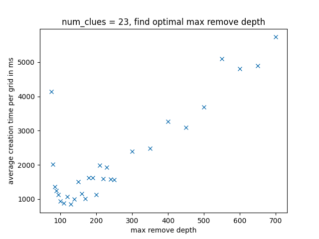
We create 100 Sudokus for each maximum remove depth and plot the average execution time over the maximum remove depth. The result below shows a similar pattern as before: at first, execution time decreases because the algorithm can backtrack more, but then it increases as the algorithm gets stuck in unfruitful branches. A value of 130 appears to be a solid default choice.
Conclusion
We explored different algorithms to solve Sudokus, check their uniqueness, generate filled grids, and create puzzles with a specific number of clues. In all cases, we used a recursive backtracking approach. The solver requires about 0.30 ms per Sudoku, while generating a complete puzzle with 23 clues takes around 1 s. Since the solver is the core component of all these algorithms, one way to improve performance would be to implement more sophisticated techniques like those described in the introduction. Another direction is to train a neural network to solve Sudokus. It will certainly be slower than classical algorithms, but still interesting to explore in a future blog post.