Implementation of CBOW (Word2vec) using PyTorch

In natural language processing (NLP), creating word embeddings—real-valued vector representations of words—is essential for tasks such as semantic search and sentiment analysis. In this blog post, we will implement and analyze the Continuous Bag of Words (CBOW) algorithm, one of the models introduced in the Word2vec paper (see [1] and [2]).
We begin by discussing the Core Ideas behind the CBOW model, followed by an explanation of the Preprocessing steps applied to the raw data. In the Training section, we present a PyTorch implementation of the model. Finally, in the Inference and Evaluation section, we explore some resulting word embeddings and interesting relationships between them.
We use several hyperparameters during preprocessing and training, with their values roughly based on [1].
The full implementation is available on my GitHub.
Core Ideas
The underlying idea of CBOW is captured by the phrase “a word is characterized by the company it keeps” (see [3]). Let’s consider the following example sentence:
“I want to learn how I can create word embeddings.”
Let’s take the word “create” as our target word. “The company it keeps”-“I”, “can”, “word”, and “embeddings”-form its context. This group of surrounding words is called the context window, and the words within it are referred to as context words.
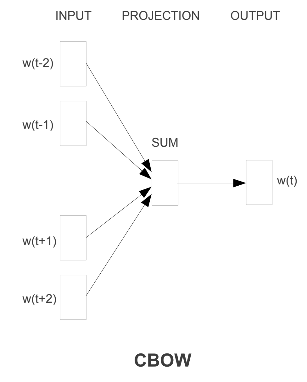
The architecture of CBOW (visualized below—taken from [1]) is designed to predict the target word from its context words. For each context window, we one-hot encode the context words. We then map these one-hot vectors to a hidden layer using a shared linear transformation without bias—that is, all context words are projected using the same weight matrix. Next, we average the resulting projected vectors to obtain a single context representation. This vector is passed through an output layer—another linear transformation without bias—producing a vector of size equal to the vocabulary size. This vector represents the logits for the target word prediction. Since we’re dealing with a multi-class classification problem, we apply a softmax to the logits and optimize the model using cross-entropy loss. Note that the architecture does not account for the distance of the context words from the target word; all context words are treated equally.
Multiplying a matrix by a one-hot encoded vector selects a specific column from the matrix. Therefore, each context word interacts with only one column of the matrix. If the algorithm learns to solve the classification problem, the information for each word must reside in a specific column of the hidden layer weight matrix. The dimension of the original one-hot encoded vector is much larger than the dimension of the matrix column. The columns of the hidden layer weight matrix are called embedding vectors, and this matrix is known as the embedding matrix.
It’s important to understand that our goal is not to predict the target word with perfect accuracy. Rather, our aim is to learn useful embedding vectors that capture both syntactic concepts, such as plurality, past tense, and opposites, as well as semantic concepts like countries, animals, and gender.
Also note that the algorithm creates features (context words) and labels (target words) from initially unlabelled data. This approach is known as self-supervised learning (see [4]).
Preprocessing
As raw training data, we use the plain text version of Simple English Wikipedia (see [5]). The goal of preprocessing is to transform raw text into pairs consisting of context words and a target word. This involves several steps:
- We split the raw text into an array of sentences.
- We remove punctuation such as commas, colons, etc., and convert all letters to lowercase.
- Each sentence is then split into a list of words, resulting in a list of sentences, where each sentence is itself a list of words.
- Next, we create the training data using the full vocabulary. We define a context window size, \(C\), which determines how many words we look ahead and behind the target word (e.g., with \(C = 4\), we can have up to 8 context words—4 before and 4 after the target word). For each sentence, we select all words as potential target words. Each target word can have up to \(2 C\) context words. This number may be smaller if the sentence is short or the target word is near the beginning or end of the sentence. If a target word has zero context words, we discard it.
- For each word that appears in the training data, we count how many windows (i.e., occurrences in target-context pairs) it appears in and record this frequency. The vocabulary is then sorted by these counts.
- To trim rare words, we retain only the \(V\) most frequent ones (with frequency defined as in step 5). All other words are removed from the training data, and any training pair that lacks a valid target word or has an empty context is discarded.
- We repeat step 5 on the filtered training data (i.e., without infrequent words) and store the updated word frequencies in our vocabulary.
- We shuffle the training data randomly to ensure that the model does not learn any unintended ordering patterns.
We use a context window size of \(C = 4\), meaning the context window consists of a maximum of 8 words. We choose \(V = 30,000\), so only the 30,000 most frequent words are considered. These choices result in 27,784,412 training pairs after applying all the preprocessing steps.
Training
Throughout this section, we explicitly state the dimensions of tensors at each step. This helps us maintain clarity and avoid confusion.
To prepare our training data in a standardized way and enable automatic batching with batch size \(B\), we implement a PyTorch Dataset (see [6]). As described in the preprocessing section, context windows may vary in size. To standardize the input, all context windows are padded to a fixed length of \(2 C\) using a special padding index of \(V\) (in our case 30,000).
As described above, in our model we need to average only the embedding vectors corresponding to the non-padded context indices. In a previous blog post, we demonstrated how to average \(M\) out of \(N\) vectors. In our case, \(N = 2 C\), while \(M\) corresponds to the actual number of context words. To apply this method, we construct a normed mask for each training sample. This mask contains ones up to the index representing the number of context words in the sample, and zeros thereafter.
The creation of the padded, fixed-length context input, as well as the corresponding normed mask, takes place within the __getitem__ method of the PyTorch Dataset. This method returns three elements: the padded context input (dimension \([B, 2 C]\)), the normalized mask (dimension \([B, 1, 2 C]\)), and the target word index (dimension \([B]\))—together forming a single training pair for our model.
Now that we’ve prepared the training data for our model, it’s time to look into the model itself. Note that PyTorch uses row vectors as inputs, meaning it follows a row-major format. This means that the matrix-vector multiplication discussed in the section Core Ideas is implemented as a vector-matrix multiplication, using the identity:
\[A \times v = v^T \times A^T \tag{1}\]Additionally, we use PyTorch’s Embedding layer (see [8]) instead of a bias-free Linear layer (see [7]).
    self.input_to_hidden: torch.nn.Embedding = torch.nn.Embedding(
        num_embeddings=vocab_size + 1,
        embedding_dim=hidden_layer_size,
        padding_idx=vocab_size
    )
The idea here is that multiplying a one-hot encoded vector with a matrix simply retrieves a specific row from that matrix. Instead of performing this operation explicitly—which introduces unnecessary computational and memory overhead—we use the Embedding layer to retrieve the row directly. We use \(H = 300\) neurons in our only hidden layer.
After embedding our padded context input of dimension \([B, 2C]\), we obtain a matrix of dimension \([B, 2C, H]\). This matrix contains the embedding vectors corresponding to each input index in the context window.
hidden: torch.Tensor = self.input_to_hidden(x)Next we have to average those vectors utilizing the pre-calculated normed mask using a vector-matrix multiplication (see the previous blog post and identity (1)). This results in a vector of dimension \([B, 1, H]\).
averaged_hidden: torch.Tensor = torch.matmul(normed_mask, hidden)Finally, we calculate the logits by the output layer using PyTorch’s Linear layer without bias.
        self.hidden_to_output: torch.nn.Linear = torch.nn.Linear(
            in_features=hidden_layer_size,
            out_features=vocab_size,
            bias=False
        )
After this last step
return self.hidden_to_output(averaged_hidden.squeeze(1))the dimension of the model’s output is \([B, V]\).
We use PyTorch’s CrossEntropyLoss (see [9]), which expects raw logits as input since it applies softmax internally.
The training is performed on an Apple M2 Max with 96 GB of RAM, leveraging Apple’s MPS (see [10]). Utilizing a batch size of \(B = 2048\) and a learning rate of \(5\) enables fast computation and stable convergence.
We calculate the average loss per epoch and plot it over the number of epochs. The loss is steadily decreasing.
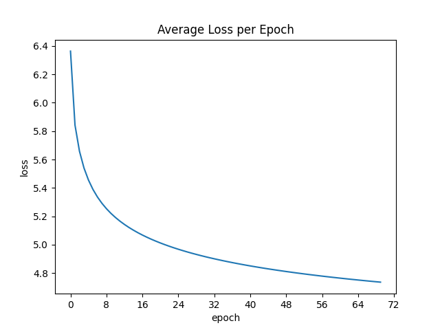
When should we stop training? It’s important to remember that our objective is not to achieve perfect predictions of the target words, but to generate word embeddings that capture the semantic and syntactic properties of words. Early in training, the embeddings improve—if they didn’t, the model architecture wouldn’t be appropriate for the task. However, as training progresses, further reductions in the prediction loss do not necessarily lead to better embeddings.
While we could define various criteria to determine when the word embeddings are good enough to stop training, this goes beyond the scope of this blog post. Instead, we simply monitor when the embeddings start to show meaningful relationships between words.
Inference and Evaluation
The word embedding vectors are found as rows in the weight matrix of the hidden layer. To measure the similarity between two embeddings, we use cosine similarity (see [11]).
We want to examine which word embedding vectors are most similar to the embedding vector of the word 'germany'. Using cosine similarity, we find that after 5 epochs, the five most similar words (excluding 'germany' itself) are:
['pens', 'france', 'bollywood', 'messenger', 'ironically']
While 'france' makes sense as it is another country, the remaining similar words appear unrelated. This suggests that the model has not yet trained long enough.
After 20 epochs, the five most similar words are:
['german', 'berlin', 'poland', 'austria', 'france']
These results indicate that the embeddings have improved. 'german' is the corresponding language, and 'berlin' is the capital. 'poland', 'austria', and 'france' are also countries, making them semantically similar to 'germany'. This suggests that the model generates useful embeddings after 20 epochs of training.
Next, we explore word analogies. In each example, the words used in the analogy are excluded from the similarity search space, and we consider only the most similar word. All evaluations are based on the model after 20 epochs of training.
Let’s analyze one of the most well-known analogy examples:
'queen' ≈ 'king' - 'man' + 'woman'
The idea is that word embedding vectors in 300-dimensional space encode abstract semantic concepts like gender. This can be extracted by subtracting the embeddings of
'woman' - 'man'
If the concept of royality is also captured in the embeddings, then adding the gender vector to the embedding for 'king' should result in a vector close to that of 'queen'.
Evaluating
'king' - 'man' + 'woman'
with our model yields
['queen']
While this shows that the word embeddings can effectively capture semantic concepts, we also evaluated the model on syntactic relationships such as:
- Opposites:
small - hot + coldresults in['large'] - Plural forms:
car - country + countriesresults in['cars']
However, other semantic and syntactic relationships do not perform as well:
- Past tense (syntactic):
listen - present + presentedresults in['breda']instead of the expected['listened'] - Capital - country analogy (semantic):
berlin - paris + franceresults in['omalley']instead of the expected['germany']
To improve these types of relationships, we would likely need to train for more than 20 epochs, adjust our hyperparameters, or use a larger raw training corpus.
Summary
In this post, we explained the concepts behind the Continuous Bag of Words (CBOW) model for creating word embeddings. We showed how to preprocess raw text into training data and provided an overview of the model’s implementation in PyTorch. Finally, we demonstrated that the embeddings encode semantic and syntactic word analogies.
Paper [1] and [2] describe techniques such as Negative sampling, Hierarchical Softmax, and Subsampling to improve computational efficiency and the quality of word embeddings. In this post, we focused on a simple implementation with a reduced vocabulary size of 30,000. For more advanced applications, open-source libraries like Gensim (see [12]) provide efficient CBOW implementations that incorporate these techniques.
Nowadays, transformer-based models—which leverage the attention mechanism—are commonly used to create more sophisticated word embeddings, as they can better capture long-range dependencies and contextual information in text (see [13]). These models can also distinguish multiple senses of a word, such as the difference between “bank” as a financial institution and “bank” as a river edge, depending on context.